The Landsat Image Mosaic of Antarctica

Robert Bindschadler, NASA Goddard Space Flight Center, Greenbelt, MD 20771, Robert.A.Bindschadler@nasa.gov

Patricia Vornberger, SAIC

Andrew Fleming, British Antarctic Survey

Adrian Fox, British Antarctic Survey

Jerry Mullins, USGS

Douglas Binnie, USGS EROS Data Center

Sara Jean Paulsen, USGS EROS Data Center

Brian Granneman, USGS EROS Data Center

Abstract

The Landsat Image Mosaic of Antarctica (LIMA) is the first true-color, high-spatial-resolution image of the seventh continent.  It is constructed from nearly 1100 individually selected Landsat-7 ETM+ scenes.  Each image was orthorectified and adjusted for geometric, sensor and illumination variations to a standardized, almost seamless surface reflectance product.  Mosaicing removed nearly all clouds producing a high quality benchmark data set of Antarctica for the International Polar Year from images collected primarily during 1999-2003.  Multiple color composites and enhancements were generated to illustrate multiple dimensions of the multispectral data including: the true appearance of the surface; discrimination between snow and bare ice; reflectance variations within saturated snow; and subtle topographic variations associated with ice flow.  LIMA is viewable and individual scenes or user defined portions of the mosaic are downloadable at http://lima.usgs.gov.  Educational materials associated with LIMA are available at http://lima.nasa.gov.

Introduction

Landsat imagery represents the oldest continuous satellite data record of the Earth’s changing surface.  Milestones in this record are represented by the production of mosaics of all the continents, except Antarctica, for epochs of 1990 and 2000 (http://glcf.umiacs.umd.edu/portal/geocover/).  The exclusion of Antarctica was dictated more by financial constraints than interest; however the rapid changes that are reported at increasing frequency and the advent of the International Polar Year increase the value of completing the suite of continental Landsat mosaics with a compilation of the southernmost continent.

 

The Long Term Acquisition Plan (Arvidson et al., 2001), used to manage the scheduling of imagery from the Enhanced Thematic Mapper Plus (ETM+) sensor on-board the Landsat-7 satellite, included the annual collection of thousands of Landsat images of Antarctica beginning in 1999.  These data form the basis of the mosaic described here.  It is referred to as the Landsat Image Mosaic of Antarctica (LIMA)

 

There were many steps required to produce the final products that are now publicly viewable and available on the web site http://lima.usgs.gov/.  These steps are described here to give interested users a more complete understanding of the reasoning and of the methods applied in the selection, processing, enhancement and management of the nearly 1100 individual images that comprise LIMA, as well as a description of the variety of mosaic products and metadata.  The primary steps include: scene selection, Level-1 processing; conversion to surface reflectance; mosaicing (cloud removal and image merging); enhancements; and web service.  Each step is described in this document.

 

The care employed in the production of LIMA has resulted not only in the first-ever true-color, high-resolution mosaic of the Antarctic ice sheet, but of a mosaic where each pixel retains accurate values of surface reflectance.  The producers of LIMA have resisted the temptation to blend scene boundaries and artificially create color balance by either uncontrolled or irreversible digital adjustments.  As a result, LIMA is more than a pretty picture that can only guide scientists to the original data, but LIMA can be used directly as a valid scientific data set.  At the same time, it serves the public’s appetite for a realistic view of the largest ice sheet and the coldest, highest and brightest continent on Earth.

Scene Selection

Landsat-7 ETM+ scenes were the preferred source of all LIMA data for three principal reasons: the geo-location of the data has been characterized to have a one-sigma accuracy of +/- 54 meters (Lee and others, 2004); extensive imaging campaigns of Antarctica undertaken soon after the April 1999 launch of Landsat-7 provided a large number of available images during the first few years of sensor operations; and the existence of a 15-m panchromatic band provided the highest spatial resolution available with any Landsat sensor.

 

Individual scenes to be used in LIMA were selected from the database of browse images representing all Antarctic Landsat-7 scenes.  The full collection of Antarctic browse images are available through the USGS (http://earthexplorer.usgs.gov/EarthExplorer/) and also were on hand at Goddard Space Flight Center having been used for manual cloud cover assessment.  Each browse image is a composite of spectral bands 5, 4, and 3 (see http://landsathandbook.gsfc.nasa.gov/handbook.html for a description of spectral characterization of the ETM+).  (Here, multiple-band composites will be identified in the usual manner of three numbers whose order represents the bands assigned to the red, green and blue channels, respectively).  These browse images are in a compressed jpeg format with an effective spatial resolution of 240 meters and provide a good indication of clouds, if present.  They do not allow the discrimination of smaller features or very thin cloud.

 

A number of factors were weighed in the decisions of which scenes to use in LIMA.  Surface coverage (therefore, minimal cloud cover) obviously was very important, but date and year of acquisition, especially of coastal scenes where a continuous sea ice cover was sought was also considered.  Selection decisions attempted to minimize large variations in sun elevation of adjacent scenes. To minimize the number of scenes, minimal overlap was sought; however, the geolocation details of individual scenes were not available.  Instead, the mean coordinates for every World Reference System-2 scene was assigned to the browse image and a public-domain software package (Geomatica FreeView V9.1) was used to compile a working version of the emerging mosaic.  In some cases, the most desirable Landsat-7 scene available contained Scan Line Corrector-off data gaps (http://landsat.usgs.gov/data_products/slc_off_data_products/index.php).  In all, LIMA contains 1073 Landsat-7 images (only 39 with SLC-off):  397 from the 1999-2000 austral summer, 75 from the 2000-2001 austral summer, 220 from the 2001-2002 austral summer, 342 from the 2002-2003 austral summer and 39 from later summers. Figure 1 illustrates the distribution of images used to generate LIMA, along with color representing the range of sun elevations.  Landsat coverage has a southern limit at 82.5oS.  To complete the continental coverage with a more pleasing visual product, data from the MODIS Mosaic of Antarctica (Haran et al., 2005) were used in a manner described later in this paper.

 

At one stage, a small number of ASTER images were considered as a viable means to replace a cloudy portion of Landsat images, however, in the final analysis, the color balancing became too difficult and the ASTER scenes were omitted from the final mosaic.

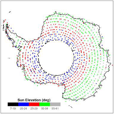
Figure 1.  Scenes selected for use in LIMA.  Dot color indicates sun elevation values are indicated by colors.  In 36 cases there were multiple images from the same path/row location: 32 with two images each and 4 with three images each.  In these cases, the highest sun elevation value is shown.

Level-1 Processing

All scenes selected for LIMA were processed from the Level-0 raw data to a Level-1T orthorectified product using the National Landsat Archive Processing System (NLAPS) processing system at EROS (details at http://edc.usgs.gov/guides/images/landsat_tm/nlaps.html).  Three digital elevation models (DEMs) were investigated to supply the elevation data necessary for orthorectification: the Radarsat Antarctic Mapping Project (RAMP version 2) DEM, (http://nsidc.org/data/nsidc-0082.html); the ICESat DEM (http://nsidc.org/data/nsidc-0304.html) and a combined radar altimeter-ICESat DEM (provided by J. Bamber). 

 

The three DEMs were intercompared at a 5 km resolution (the supplied post spacing of both the ICESat and radar altimeter-ICESat DEMs).  Differences were examined to help discern how they might affect the orthorectification process in different parts of Antarctica.  The deciding factors were coverage and accuracy in mountainous regions.  The ICESat DEM was not complete to all edges of the continent, and the radar altimeter-ICESat DEM was not able to include the extreme topographic variations of the mountainous regions.  Because Landsat’s field of view is nadir and near-nadir, ortho-rectification corrections are largest in areas of high relief and at the scene edges.  For these reasons, the RAMP version 2 DEM, which also is available on a much finer 200-m spacing, was selected for orthorectification in the NLAPS processing stream.

Conversion to Surface Reflectance

Many steps were required to convert the radiance measured at the ETM+ sensor to an accurate value of surface reflectance.  These are discussed below in the order they were applied to the NLAPS-processed data. 

Saturation Adjustment

The high reflectance of snow at optical wavelengths can saturate the ETM+ sensor.  Saturation radiance thresholds vary by band, by gain setting (High or Low) and by illumination geometry (sun elevation and surface slope).  Table 1 indicates the saturation radiance, L_max, for ETM+ bands (both High and Low gain setting).

 

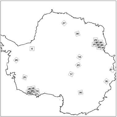
Table 1. ETM+ Spectral Radiance Range (W/(m² * ster * mm)), from Table 11.2 in http://landsathandbook.gsfc.nasa.gov/handbook/handbook_htmls/chapter11/chapter11.html

 

The spectral reflectance of snow varies with the specific type of snow (primarily snow grain size and wetness).  In general, snow is most reflective in Band 1, decreasing through Bands 2 and 3, decreasing to even lower values in Band 4 and decreasing to very low values in Bands 5 and 7 (see Dozier and Painter, 2004, for a review of multispectral remote sensing of snow).  As snow ages, the snow grain size increases, and reflectance decreases at all optical wavelengths. 

 

Failure to adjust for saturation will cause saturated image pixels to be converted to an incorrect spectral reflectance that is lower than the actual reflectance, and produce improper colors in multi-band composite images.  Saturation adjustment is completed before any other adjustment because it is easiest to identify saturation at this early stage of image processing by the test condition that a pixel value is saturated (Digital Number (DN) = 255, the maximum value for the 8-bit data range of ETM⁺).  DNs correspond to a band-specific scaled radiance value, but the conversion to radiance is made after the saturation adjustment discussed here. 

 

Saturation values (DN=255) of a given pixel are adjusted to DN values greater than 255 by applying a predetermined spectral ratio to an unsaturated band value at the same pixel.  The appropriate spectral ratio was determined by examining 27 Landsat scenes across Antarctica that were selected to provide a variety of surfaces, a variety of sun elevation values and all three gain combinations of spectral bands used for ETM+ acquisitions of Antarctica (see Figure 2 and Table 2).    

 

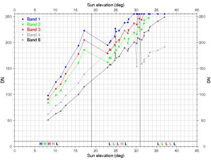
Figure 2. Location of 27 Landsat ETM+ scenes used to determine empirical relationships for saturation adjustment and non-diffusive reflectance of LIMA images.  Numbers in scene outline boxes refers to sun elevation at center of each scene.

 

The distribution of DN for snow pixels within each image was checked to be normally distributed and the DN of the histogram peak for each band in each scene was identified.  The DN value of the histogram peak depended strongly on sun elevation, with lower DN values for lower sun elevations (Figure 3).  Band 1 always had the highest snow-histogram maximum DN value, Band 3 was somewhat lower, then Band 2, followed by Band 8.  The relative position of Band 4 depended on its gain setting—the gains of Bands 1, 2 and 3 were always either all High or all Low, depending on sun elevation, while Band 4 was switched independent of any other band.  Band 8 always remained at Low gain.  Bands 5 and 7 were not considered.  These interband relationships are consistent with snow spectra of aging snow collected in the field (Dozier and Painter, 2004). 

 

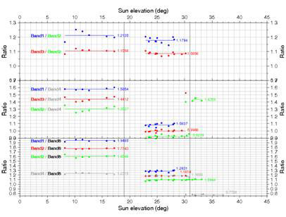
Figure 3.  DN of the snow histogram maximum plotted versus sun elevation for each band of the 27 ETM⁺ scenes indicated in Figure 1.  Gain settings for Bands 1-4 and 8, indicated by H and L along the bottom of the plot, were tied to sun elevation.

 

Band-to-band spectral ratios were calculated from the data plotted in Figure 3.  They are very consistent for the same gain combination and indicate no dependence on sun elevation (Figure 4).  These ratios are also given in Table 2.  Their consistency forms a sound basis for our saturation adjustment methodology. 

 

 

Figure 4. Band-to-band ratios versus sun elevation derived from Figure 3 values.

 

 

Table 2.  Spectral band ratios of DN for snow regions of the 27 sample scenes indicated in Figure 2.  Gain settings are given as High (H) or Low (L) in order of bands 1, 2, 3, 4, 8.

Band Ratio	HHHHL	LLLHL	LLLLL
Band1/Band2	1.2130	1.1794	1.1794
Band3/Band2	1.1058	1.0858	1.0858
Band1/Band8	1.9460	1.2831	1.2831
Band2/Band8	1.6048	1.0944	1.0944
Band3/Band8	1.7743	1.1814	1.1814
Band4/Band8	1.2315	1.1806	0.7728

 

In applying this saturation adjustment to the LIMA scenes, every pixel in every scene was examined for saturation in the following band order: 1, 3, 2, 4.   If saturation was identified (DN=255), then the pixel’s value in Band 2 is used along with the appropriate spectral band ratio (depending on the relative gain settings, see Table 2) to adjust the saturated DN value to a higher value based on the DN value of the unsaturated band.  If Band 2 is also saturated, then Band 8 is used, with the appropriate spectral ratio (see Table 2).  

Sensor Radiance to Surface Reflectance Conversion

The ETM+ sensor was frequently calibrated to maintain an accurate conversion of the DN value to the at-sensor radiance (see Chapter 9 of the Landsat-7 Science Data Users Handbook at http://landsathandbook.gsfc.nasa.gov/handbook/handbook_toc.html).  These calibration coefficients are included in the header files of every NLAPS-processed Landsat scene.  The conversion from DN to at-satellite radiance is accomplished by applying the following equation:

L(λ) = {[L_max(λ) – L_min(λ)]/255} * DN + L_min(λ)                                                                            (1)

Where L(l) is the spectral radiance at the sensor’s aperture, and L_min(l) and L_max(l) are the spectral radiances that correspond to DN=0 and DN=255, respectively (see Table 1).  Radiances are given in W/m²*ster*mm. 

From these calibration values, the conversion of at-sensor radiance to planetary reflectance follows from:

                                                       (2)

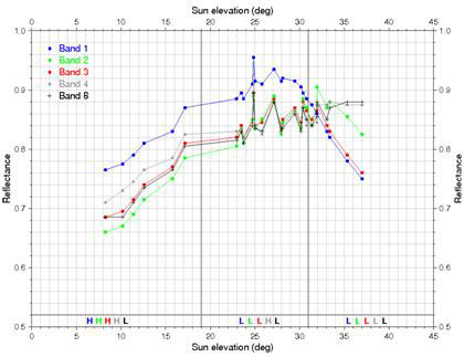
Where r is planetary reflectance, d is the Earth-Sun distance (in AU), E_s(l) is the mean solar exoatmospheric irradiance, and J_s is the solar zenith angle (in degrees) (see Chapter 11 of the Landsat-7 Science Data Users Handbook).

 

Converting planetary reflectance to surface reflectance usually involves the use of an atmospheric scattering model.  Such models require input values of atmospheric water vapor and aerosols.  The atmosphere over most of the Antarctic continent is very cold, minimizing the amount of water vapor, and very clean, minimizing the concentration of aerosols.  The assumption made here is that these atmospheric corrections are negligible and the planetary reflectance is a good approximation of the surface reflectance.

 

The cosine dependence of the surface brightness results from the fact that the illuminated surface area per solid angle of incoming solar radiation varies with the cosine of the sun elevation angle.  This situation strictly only applies for a horizontal surface.  For sloping surfaces, the slope component in the direction of the solar illumination must be added to the sun elevation angle.  It is this additional factor that allows the surface topography of the ice sheet to be visually discerned by brightness variations in Landsat images of the ice sheet.  Calculated reflectance values in excess of 100% are not uncommon in sloping snow covered terrain when the surface slope is not included in Equation 2.

Local Sun Elevation Adjustment

At high latitudes, the local sun elevation varies significantly (i.e., a few degrees) across a Landsat scene.  This requires the solar elevation in Equation 2 to be the local sun elevation angle at each pixel and not the scene-center value.  The local sun elevation angles are calculated by using a solar ephemeris to calculate the solar elevation at each of the four scene corners for the time and date of the scene center.  The solar elevation at each pixel is then calculated using a bi-linear interpolation of the four scene-corner sun elevations.

Correction for non-Lambertian Reflectance

The DN-to-surface reflectance conversion employed by Equation 2 assumes the reflectance character of the surface is Lambertian and that the Landsat sensor views the surface from directly overhead.  While the second assumption is generally valid, even at the image edges, the first is not. At progressively lower sun elevations, snow deviates from the properties of a Lambertian, perfectly diffusive reflector due to increasing forward scattering (Warren et al., 1998, Masonis and Warren, 2001). 

 

Field studies of this effect provide limited quantitative estimates of this non-Lambertian effect.  We also draw upon an empirical form of this relationship based on the same 27 Landsat scenes referenced above (Figure 2).  Figure 5 shows how the surface reflectance, calculated from Equation 2, varies with sun elevation.  In this figure, the Band 1 reflectance decreases as sun elevation increases beyond 27 degrees and Band 2 and 3 reflectances decrease as sun elevation increases beyond 31 degrees due to saturation.  These decreases are not a real effect, rather, they are the result that a saturated sensor reading of 255 underestimates the actual at-sensor radiance and this underestimate of radiance is converted, through Equation 2, to an underestimate of reflectance. 

Figure 5. Surface reflectance versus sun elevation for the 27 Landsat scenes indicated in Figure 2.  Surface reflectances are calculated from Equation 2 without any saturation adjustment applied.

 

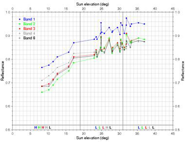
Saturation adjustment, as described above, corrects the artificial surface reflectance decrease at higher sun elevations (Figure 6).  What remains is the non-Lambertian effect of decreasing surface reflectance as sun elevation decreases.  This affects nearly all sun elevations in the LIMA data set, becoming marginal for sun elevations above 30 degrees. 

 

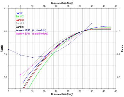
Figure 6. Surface reflectance versus sun elevation (see Figure 5) after saturation adjustment.

 

Our adjustment for the non-Lambertian reflectance effect takes the form of an adjustment ratio for each spectral band.  The purpose of this adjustment is to increase the calculated reflectances at lower sun elevations to what the reflectance would have been if the surface were a Lambertian reflector or if they had been illuminated with the same solar elevation. These ratios were determined initially by fitting quadratic curves to the non-saturated data pairs of surface reflectance versus sun elevation, i.e. the data in Figure 6 were fitted by quadratic curves, and dividing those fitted values by a “standard” reflectance value for each band.  The initial ratios contained slight biases that were subsequently removed by fitting a line to the adjusted reflectances and modifying the ratios so that the mean of the adjusted reflectances for each band matched the standard reflectances.  The standard reflectance values were chosen based on the observation that our derived reflectance values agreed with field data at 31 degrees solar elevation (Masonis and Warren, 2001).  These values are given in Table 3.  The field data are limited to 600nm wavelength—in the absence of other field data we assume here that a similar correlation applies at all wavelengths.  The resulting ratio values are shown in Figure 7 along with a similarly calculated set of ratios for the field data.  Surface reflectances calculated for saturated pixels are included in Figure 6, but excluded from the quadratic fits and the non-Lambertian adjustment ratios.

 

Table 3. “Standard” spectral reflectance for snow

Band 1	0.9362
Band 2	0.8694
Band 3	0.8697
Band 4	0.8599
Band 8	0.8556

 

Figure 7. Non-Lambertian adjustment ratio versus sun elevation derived from 27 Landsat scenes shown in Figure 1 and for field data (from Masonis and Warren, 2001).

Reflectance Normalization

Our final adjustment to surface reflectance is not physically based, but motivated by the desire to produce a visually consistent mosaic by eliminating visually distracting edges between adjacent scenes.  LIMA unavoidably includes scenes with slight differences in actual surface conditions.  To minimize reflectance “offsets”, we perform a final adjustment to match the mean snow reflectance of each scene to the “standard” spectral reflectances described above (cf. Table 3). 

 

To implement this final adjustment, the reflectance histogram of each scene is quantified for each band using a reflectance binning interval of 0.004.  Once quantified, the histogram bin above 0.5 reflectance that has the greatest number of occurrences is determined, and the reflectance value of that bin is compared with the corresponding “standard” spectral reflectance.  A “reflectance normalization” ratio (equal to the “standard” reflectance divided by the actual reflectance) is then applied to the entire scene to force the maximum reflectance occurrence to match the “standard” spectral reflectance.  A ratio approach is used to minimize the changes for lower reflectance regions, e.g. rock. 

 

After accounting for all of the above adjustments, the actual equation that is applied is of the same form as Equation 2, but modified to the following:

                                                        (3)

where f_NL is the adjustment ratio for non-Lambertian reflectance, and f_SR is the histogram-based “reflectance normalization” adjustment ratio to the “standard” snow reflectances.  These spectral reflectance shifts are recorded in an ancillary data file to ensure that the adjustments are preserved and are available to LIMA users in a metadata file.

 

Reserving the non-physical adjustment to the last of the series of adjustments described in this section provides a measure of the success of the earlier adjustments in creating a high-quality data set of uniformly treated scenes.  In practice, most LIMA scenes did not require any significant normalization adjustment.  Of the 4292 values of f_SR (4 bands for each of 1073 scenes), only 9% required a “reflectance normalization” adjustment ratio greater than 1.05 or less than 0.95, mostly in Band 4.

Mosaicing

Once the individual scenes have been adjusted, they were mosaiced together using customized software developed by ITT VIS to be used within the ENVI image processing environment.  The mosaicing procedure began by determining a stacking order of scenes (the single value of any pixel comes from the uppermost scene with a value for that pixel) and then omitting unwanted portions of scenes, such as clouds, to allow preferred portions of scenes lower in the stack to show through.  In practice, many clouds present in the selected scenes were effectively removed by ensuring that another scene, with corresponding cloud-free pixels was placed higher in the image stack. 

 

Although every attempt was made to normalize the reflectances of all the scenes, the adjustments detailed above were only performed to entire scenes.  There were a few instances where there were reflectance variations within a scene that caused a visual mis-match between it and all its neighboring scenes.  In this case, judicious trimming of scene boundaries was employed to minimize these visually disruptive scene-to-scene jumps in reflectance.  Any residual mismatch in adjacent scene color balance was removed by applying band-specific adjustments based on local histogram statistics.  These adjustments are recorded in the LIMA metadata and were required for only 62 of the 1073 scenes.

 

The most difficult area to produce a visually smooth mosaic was around the ice sheet margin where temporal variations of the sea ice pack and changes in the extent of ice shelves produced inevitable discontinuities in adjacent scenes, but inevitably some edges remain.  Again, these were minimized through suitable trimming and stacking of adjacent scenes.  Further there are a small number of areas where it was not possible to identify suitable cloud free imagery and patches of cloud are still present. As more suitable imagery of these regions becomes available these portions will be updated.

 

The data volume of so many scenes required that the mosaic be prepared in a series of 25 smaller blocks, each composed of 24 to 76 individual scenes.  This “building block” structure was incorporated into the mosaicing software allowing blocks, once completed, to be combined through output instruction files into a larger mosaic.  In fact, the full continental mosaic never existed as a single file, rather only as a “virtual mosaic”—a series of separate image files (each a combination of a few blocks) linked by a control file that could guide subsequent operations on the mosaic exactly as if the mosaic actually did exist in a single file.  This approach avoided the need for extremely large files and the associated storage and file input/output problems that can accompany very large files.

 

From this mosaicing operation and the virtual mosaics that were created (one for every spectral band), a series of geotiff tiles were created that covered the entire continent.  170 geotiff tiles were produced because the maximum allowable size of a geotiff file is 2 gigabytes.  The tile pattern was created to ensure that the production of the various multiband composites and contrast-stretched enhancements (described in the next section) would also not exceed the geotiff size limitation using the same tile arrangement.

Data Precision

Any description of a new data set requires a careful explanation of data precision.  This topic perhaps is best presented at this juncture between the end of the data processing procedures and the beginning of the generation of display products.  Much earlier, it was mentioned that the NLAPS processing of individual scenes produced multiband data with 8-bit precision.  An 8-bit representation imposes an upper bound to the accuracy due to the number of quantization levels.  This quantization constraint is consistent with the noise levels of the multispectral bands and of the panchromatic band of the ETM+ sensor, approximately 1 DN and 2 DN, respectively (Scaramuzza et al., 2004).

 

All of the post-NLAPS processing steps described above carried a 16-bit level of precision to the various data adjustments.  This was important to allow these refinements to have their full effect and not be lost in truncations or roundings of the very last bit of the 8-bit data values.  With the extra range afforded by 16-bit data, the spectral reflectances are calculated to the nearest 1/100 % (i.e., a value of 10,000 represents a reflectance of 100%).  To preserve the highest level of LIMA image quality, the 16-bit mosaics of each spectral band are available. 

 

Most computer displays require 8-bit gray-scale signals, or 24-bit color signals (three bands for the red, green and blue color guns, each in 8-bit).  For this reason, the various display products described below are all generated as 8-bit single band, or 24-bit color composites. 

Enhancements

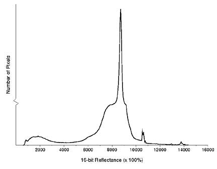
Digital imagery enables enhancement of the visual representation of the digital data through the use of different assignments of the original data values to those displayed on a computer monitor.  These methods are very appropriate to LIMA where so many of the snow surface features occur in a very narrow range of reflectances and dark rock lies adjacent to bright snow.  This section describes the various techniques employed to allow the user to see more of the digital content of LIMA.  Ultimately, the availability of the LIMA data in 16-bit digital form allows users unlimited possibilities for additional enhancements.

 

Figure 8 is a histogram of a typical scene fully processed for LIMA.  It includes a very large but narrow peak for snow pixels that dominate the Antarctic surface (note the scale change on the vertical axis), a much smaller peak at low reflectance (corresponding to dark rock), includes pixels with reflectances between these two peaks, as well as some pixels with reflectances above 100% (10,000 in 16-bit values).  Few reflectances exceed 160% (16,000 in 16-bit values) and no data value is less than 1 (the value zero is reserved to represent “no data”).  The reflectance at the histogram peak is 87.28%.  These histogram values become important in the enhancements to follow.

 

 

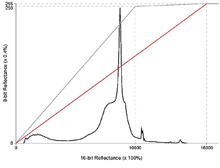
Figure 8. Representative histogram of 16-bit reflectance values for a LIMA scene.  There is a scale change on the vertical axis to capture both the full extent of the major histogram peak as well as the detail at other reflectance values. 

Pan-Sharpening

The LIMA enhancements begin with “pan-sharpening” to increase the spatial resolution of the spectral bands.  This involves applying the finer spatial variations of the 15-meter spatial resolution panchromatic band (Band 8) to the 30-meter resolution narrower spectral bands (Bands 1-4).  A key characteristic of the spectral and panchromatic bands is that they are coregistered.  The upper left corners of the upper left pixels of each band are co-located.  From that common point, all pixels of all the 30-meter spectral bands are also co-located.  The panchromatic band has its 15-meter pixels nested within the 30-meter pixels such that every 2 x 2 square of panchromatic pixels matches the location of a 30-meter pixel.

 

This convenient alignment is used to increase the resolution of the spectral bands with a simple algorithm.  Each 30-meter spectral band pixel is subdivided into four 15- meter pixels.  For a specific pixel, let S be the initial pixel value and let s1, s2, s3 and s4 be the values to be assigned to the 15-meter subdivided pixels.  The four panchromatic pixel values (p1, p2, p3, p4) are averaged together to a mean value of P and the spectral values are then calculated as:

s1 = S * p1/P

s2 = S * p2/P

s3 = S * p3/P

s4 = S * p4/P

 

This formulation has the additional property that the original 30-meter spectral values can be recovered by averaging the pan-sharpened 15-meter pixels.

Base Composites

Color composites are produced by converting the single-band, pan-sharpened 16-bit values at each pixel to 8-bit single band values and combining three bands into a 24-bit color product.  An 8-bit number cannot be larger than 255 (starting at 0).  To compress the 16-bit range of reflectances into this narrower range, each 16-bit reflectance value (in hundredths of percent) between 0 and 10,000 is divided by 40.  Thus, 100% reflectance is converted to a value of 250.  To convert any 8-bit value to the corresponding reflectance value (in percent), it must be divided by 2.5.  Reflectances in 16-bit data above 10,000 (and below the maximum value of 16,000) are converted to 8-bit values between 250 and 255. 

 

The specific equations used are:

 

r = R/40                                   0<R<10,000

r = R/1200 + 241.67;       10,000<R<16,000

r = 255;                                       16,000<R

 

where R is the 16-bit value and r is rounded to the nearest 8-bit value excluding r=0.  The difference between the divisor of 40 for the reflectance range 0-100% and the divisor of 1200 for reflectances above 100% means that very bright reflectances (such as can occur on the sun-lit sides of steep snow-covered mountains) are highly compressed into a very narrow range of values in the 8-bit representation of LIMA.  An example of this effect is illustrated later and a later enhancement is designed to relax this data compression of very bright values at the expense of compressing darker data pixels.

 

Figure 9 illustrates this 16-bit to 8-bit conversion by the thin black line that matches any 16-bit number on the horizontal axis with the converted 8-bit number on the vertical axis.

 

Figure 9.  Histogram of typical LIMA 16-bit reflectances with the thin black line showing the conversion from the16-bit reflectance values to 8-bit reflectance values for the basic (no-stretch) enhancement, and the red line showing the conversion from the16-bit reflectance values to 8-bit reflectance values for the 1X (sunglasses) enhancement.

 

To preserve the color balance through this 16-bit to 8-bit conversion (and all the others that follow), it is applied only to Band 2 (green).  The corresponding values for the other bands (1, 3 and 4) are calculated by scaling the enhanced (8-bit) values by the ratio of the unenhanced (16-bit) reflectances.  Thus, if G and g are the unenhanced and enhanced values of Band 2, respectively, and B is the unenhanced value of Band 1, then the enhanced value of Band 1, b, is:

 

b = g * B/G

 

Similar equations hold for Bands 3 and 4.

 

Two “base”, i.e., unenhanced, products are produced from this 16-bit to 8-bit conversion of spectral Bands 1 through 4.  One is a combination of Bands 3, 2, and 1 into the red, green and blue channels.  Because of the spectral locations of these bands, this produces a true-color representation of LIMA data.  The second base composite is a combination of Bands 4, 3, and 2 into the red, green and blue channels.  This “false-color” combination holds some advantage over the true-color composite for discriminating between bare ice (appearing more blue) and snow (that still appears white).  Figure 10 illustrates a sample of each composite.

 

 

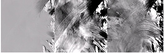
Figure 10.  Comparison of the 321 (left) and the 432 (right) color composites for a region of North Victoria Land in East Antarctica.  Each subimage is 7 km across.

Enhancements

Subtle variations of the LIMA data set are not apparent visually in the base composites because the human eye is not capable of resolving 256 different shades of any color.  Digital enhancements can be constructed to highlight selected portions of the reflectance range so they can be seen more easily.  To make these subtle details viewable, a set of digital enhancements have been performed on the 16-bit bands prior to combining them into additional true-color (321) and false-color (432) composites. 

 

The first enhancement is designed to accentuate very bright reflectances (over 100%) that were strongly compressed in the base composites.  To accomplish this, the bilinear enhancement of the base composites described above is modified to a single divisor of 62.745(=16,000/255).  This enhancement has two major results.  One is that the reflectances above 100% are now represented by a larger portion of the 0-255 range of 8-bit values, allowing the spatial variations to be seen more easily.  The other result is that the reflectances in the 0 to 100% range will not only be distributed over a smaller portion of the 0-255 8-bit range than before, thus sacrificing some visual detail, but they will also be represented by lower values, making these pixels appear darker than in the base composites.  The specific equations used are:

 

r = R/62.745                0<R<16,000

r = 255;                            16,000<R

 

where R is the 16-bit value and r is rounded to the nearest 8-bit value excluding r=0. 

 

The red line in Figure 9 illustrates this enhancement and helps illustrate why the snow surfaces appear darker with the enhancement than in the base composites.  An illustration of the 1X enhancement is given in Figure 11.  This enhancement acts much like wearing a pair of sunglasses and so is termed the “sunglasses” enhancement.  Both true-color (321) and false-color (432) composites are formed from these enhanced bands. 

 

 

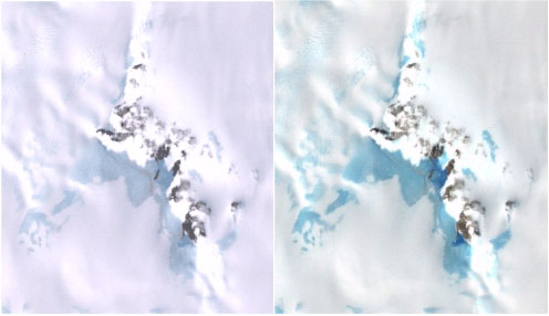
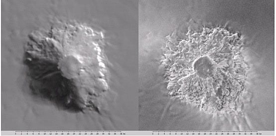
Figure 11. LIMA sub-image of Mt. Takahe in West Antarctica with the 321 true-color composite (left) and with the 1X “sunglasses” enhancement (right).  Details of the sun-facing slope appear “overexposed” in the left sub-image and more visible in the 1X enhancement.

 

The remaining enhancements are all aimed at increasing the visual appearance of detail in the flatter ice sheet surface which, in terms of relative area, dominates Antarctica.  These surfaces fall into the range of reflectances in the large histogram peak (see Figure 8) whose central peak of 87.28% reflectance converted to an 8-bit value of 139 in the previous (1X) enhancement.  This value is retained in these remaining enhancements while the strength of the stretch (i.e., the slope of the line in the histogram figures) is increased by factors of 3X, 10X and 30X.  To use more of the 8-bit range to display these details requires that some other portions of the full range of 16-bit reflectances be compressed to increasingly narrower ranges of 8-bit values.  We define a tri-linear enhancement where the middle linear segment is centered on this 87.28% reflectance (at an 8-bit value of 139) and pivoted to various slope values.  This central linear segment is limited to the 8-bit range from 25 to 230.  On either side of this central segment, another linear segment converts the 16-bit values to 8-bit values of 1 to 25 for low reflectances, and 230 to 255 for high reflectances. 

 

In the 3X case, called the “low-contrast” enhancement, the specific equations applied are:

 

r = R/253.76;                                        0<R<6344

r = R/20.915 – 278.3075;            6344<R<10,631

r = R/214.76 + 180.498;           10,631<R<16,000

r = 255;                                                  16,000<R

 

where R is the 16-bit value and r is the 8-bit value excluding r=0.  Figure 12 illustrates the nature of this enhancement superimposed on the representative histogram.

 

 

Figure 12.  Histogram of typical LIMA 16-bit reflectances showing the conversion from the16-bit reflectance values to 8-bit reflectance values for the 3X “low-contrast”, 10X “medium-contrast”, and 30X “high-contrast” enhancements.

 

The “medium-contrast” enhancement provides an even stronger (10X) stretching of the dominant ice-sheet surface reflectances to reveal even finer details of the snow surface.  The specific equations applied are:

 

r = R/320.52;                                        0<R<8013

r = R/6.2745 -1252.03;                    8013<R<9299

r = R/268.04 + 195.307;              9299<R<16,000

r = 255;                                                 16,000<R

 

where R is the 16-bit value and r is the 8-bit value excluding r=0.  Because the differences between the true-color and false-color composites are so slight, only a true-color composite is produced.

 

The “high-contrast” enhancement applies the strongest (30X) contrast stretch to the 16-bit data to show the most subtle features contained in the imagery.  The specific equations applied are:

 

r = R/339.60;                                        0<R<8490

r = R/2.0915 – 4034.075;              8490<R<8918

r = R/283.28 + 198.519;             8918<R<16,000

r = 255;                                                 16,000<R

 

where R is the 16-bit value and r is the 8-bit value excluding r=0.  Once again, only a true-color composite is produced.

 

In each of these contrast enhancement cases, the equations are applied to the 16-bit, pan-sharpened Band 2 mosaic.  Other bands are converted to 8-bit values to preserve the color balance (as described above) and true-color (321) and false-color (432) composites are generated.  Because the middle segment of this enhancement is pivoted on the same value as in the first enhancement (Figure 9), the overall ice-sheet appearance of the contrast enhancements will appear similar to the 1X enhancement, i.e. darker than the base composites, but that areas that were either very dark or very bright in the base composites will appear even darker and even brighter, respectively, in each contrast enhancement. An example of the successively stronger contrast enhancements is shown in Figure 13.

 

 

Figure 13.  Sample of the contrast enhancements progressing (left to right) from no enhancement to 3X, 10X and 30X, for a portion of the megadune area of East Antarctica.  Each image is 12 km on a side.

 

Because LIMA is also available as 16-bit data product, users can apply a nearly limitless variety of enhancements and image processing procedures tailored to the user’s interests and objectives.  An example of this is shown in Figure 14 where a customized enhancement is applied to draw out details of ice flow features in a region where two glaciers exit the Transantarctic Mountains and join as they enter the Ross Ice Shelf.

 

 

Figure 14.  Sample of the customized enhancement of a region of two merging glaciers showing the ability of the 16-bit LIMA data to reveal significant surface detail.  Left sub-image is the region in the 1X enhancement, middle sub-image is after a strong enhancement, and the right sub-image is the same region cropped from the MODIS Mosaic of Antarctica (MOA).  Each image is 110 km on a side.

 

Complementary Mosaics

Although LIMA represents a significant addition to the ability to “see” Antarctica, we view it as complementary to other existing mosaics.  We have already mentioned the MODIS Mosaic of Antarctica (Haran et al., 2005) and used it in the comparison in Figure 14.  MODIS data have lower spatial resolution, but a wider field of view and more radiometric resolution.  This often enables clearer views of extensive surface features where LIMA scene edges might begin to interrupt the larger scale view.  On the other hand, LIMA’s spatial detail can be instructive in probing the smaller scale limits of MOA. 

 

Both LIMA and MOA were preceded by the continental scale mosaic of Antarctica created from synthetic aperture radar data collected by Radarsat (Jezek et al., 2001).  Speckle reduces the effective spatial resolution of the Radarsat mosaic to close to 100 meters, but the dominant appearance of this mosaic is an emphasis on sharp edges, such as surface crevasses or rugged topography.  This emphasis can be exceptionally useful in a variety of glaciological and geological studies and, again, the combination with LIMA’s visual representation of the surface can introduce a high degree of synergy in linked examinations of these data sets.  Figure 15 illustrates the MOA and Radarsat mosaics’ view of Mount Takahe to compare with the LIMA view in Figure 11.

 

 

Figure 15.  Sub-images of Mount Takahe, West Antarctica, in the MODIS Mosaic of Antarctica (left) and the Radarsat mosaic of Antarctica (right).  Each image is approximately 48 km on a side.

 

Web Services

The World Wide Web provides an excellent medium for researchers and the public to interact with LIMA.  The primary user interface (http://lima.usgs.gov) includes a viewer that supports scrolling and zooming functions that allow users to either explore the data on-line or to download subsets of specific LIMA enhancements.  Individual scenes used in the mosaic can be identified and downloaded separately as multispectral data at the NLAPS product level or as a 16-bit reflectance product.  Eventually, data subsetting based on user defined areas are intended.

 

The USGS web site also includes the Interactive Atlas of Antarctic Research, where a variety of other map-based data layers can be displayed simultaneously with LIMA by employing a provided transparency parameter. Useful non-LIMA data layers, such as other continental data sets (e.g., the MODIS Mosaic of Antarctica, or the Radarsat Mosaic of Antarctica) or localized data sets (e.g., coastline vector files, station locations, digitally scanned maps) can be layered with additional transparencies applied. 

 

An associated web site (http://lima.nasa.gov) focuses on education and outreach activities using LIMA as a platform.  At this site, there are descriptions and examples of how researchers use digital imagery, including lesson plans and materials for educators, and a useful link to the Antarctic Geographic Names database that supports searches on user-specified names and a link back to LIMA to display a centered-view of the feature in LIMA.  A flyover of the Ross Island, Dry Valleys area is also available with more three-dimensional visualizations available at http://svs.gsfc.nasa.gov/  (search on keyword “lima”).  All of these sites aim at to use LIMA to make Antarctica more familiar to the public and to enhance the scientific research of this continent.

Summary

The Landsat Image Mosaic of Antarctica represents a major advance in the ongoing digital record of our planet.  It provides researchers and the public with the first-ever high spatial resolution, true-color mosaic of this continent.  The nearly 1100 images used to construct the mosaic are now freely available as individual scenes, as a nearly seamless mosaic and in a variety of enhancements designed to highlight meaningful details of the surface.  Most of the images fall within the four-year period from 1999 to 2003, making this data set an important milestone in the accelerating evolution of the Antarctic continent.  As such, LIMA is a major benchmark data set contribution to the 2007-2008 International Polar Year.

 

The processing of the image data was held to a rigorous standard that preserved the values of each pixel through a complex series of deterministic adjustments.  Image data were initially processed from raw data and orthorectified.  Thereafter, a combination of sensor calibrations and empirically-determined adjustments converted the data to surface reflectance values in multiple spectral bands.  The precise adjustments for each image are available as metadata.  This rigor sets a new standard in the quality and value of large-scale mosaics with Landsat imagery. 

 

Enhancements of these data included pan-sharpening to increase the spatial resolution, and an assortment of contrast stretches to illuminate different features of the Antarctic continent.  It is anticipated that the variety of enhancements will supply any user with a sufficiently wide range of readily accessible views of LIMA to facilitate both curiosity-driven exploration of Antarctica and scientific research.  Other enhancements can be customized by the user by acquiring either the 16-bit mosaic data or beginning with any of the above-described enhancements.   

Acknowledgements

This project was supported by the National Science Foundation through grants #0541544 to NASA and #0233246H to USGS and by the British Antarctic Survey.  It is regarded as a major benchmark data set of the International Polar Year.

References

Arvidson , T., J. Gasch and S.N. Goward, 2001. Landsat 7's long-term acquisition plan - an innovative approach to building a global imagery archive, Remote Sensing of Environment, Vol. 78, No. 1-2, p. 13-26. 

 

Dozier, J. and T.H. Painter, 2004.  Multispectral and Hyperspectral Remote Sensing of Alpine Snow Properties, Annual Reviews of Earth and Planetary Science, Vol. 20, p. 465-94.

 

Haran, T., J. Bohlander, T. Scambos, T. Painter, and M. Fahnestock compilers. 2005, updated 2006. MODIS mosaic of Antarctica (MOA) image map. Boulder, Colorado USA: National Snow and Ice Data Center. Digital media.

 

Jezek, K., and the RAMP Product Team, 2002. RAMP AMM-1 SAR Image Mosaic of Antarctica.  Fairbanks, AK: Alaska SAR Facility, in association with the National Snow and Ice Data Center, Boulder, CO.  Digital media.

 

Lee, D.S., J.C. Storey, M.J. Choate, and R.W. Hayes, 2004.  Four Years of Landsat-7 On-Orbit Geometric Calibration and Performance, IEEE Transactions on Geoscience and Remote Sensing, Vol. 42, No. 12.

 

Masonis, S.J. and S.G. Warren, 2001.  Gain of the AVHRR visible channel as tracked using bidirectional reflectance of Antarctic and Greenland snow, International Journal of Remote Sensing, Vol. 22, No. 8, pp. 1495-1520.

 

Scaramuzza, P.L., B.L. Markham, J. A. Barsi, and E. Kaita,  2004.  Landsat-7 ETM⁺ On-Orbit Reflective-Band Radiometric Characterization, IEEE Transactions on Geoscience and Remote Sensing, Vol. 42, No. 12,  p. 2796.

 

Warren, S.G., R.E. Brandt and P. O’Rawe Hinton, 1998.  Effect of surface roughness on bidirectional reflectance of Antarctic snow, Journal of Geophysical Research, Vol. 103, No. E11, pp. 25,789-25,807.